
R for bioinformatics (and more!)
1. Introduction
This page wis generated using Rmarkdown. It shows code in blocks, and the results of running that code below it.
Blocks that start with ## are the output.
The code shown here is replicated from the scripts we go through in the workshop. We will cover in detail each section, in tandem with our slides.
The purpose of posting this content is for reference only, it is not intended to be a stand-alone tutorial.
1.1 Objects
There are a lot of different types of objects in R. Each is useful for different purposes.
# Numbers
(0.013 + 0.008 + 0.011) / 3
## [1] 0.010666671.2 Variables
Variables let us store objects with a name, and make them easy to access later. We can use variables in the same way we use the objects they refer to.
We can view a variable x with print(x), or by simply writing x
num_snails <- 3

speed_snail1 <- 0.013
speed_snail2 <- 0.008
speed_snail3 <- 0.011

(speed_snail1 + speed_snail2 + speed_snail3) / num_snails
## [1] 0.01066667# Numeric
a <- 1
print(a)## [1] 1# Strings (of characters)
b <- "my snail is the fastest!"
print(b)## [1] "my snail is the fastest!"1.3 Functions
# c() is a function, and it returns a vector
snail_speeds <- c(speed_snail1, speed_snail2, speed_snail3)
print(snail_speeds)
## [1] 0.013 0.008 0.011# we can use the mean() function to get the average of the vector
mean(snail_speeds)## [1] 0.01066667# we can even create our own functions
fastest_snail <- function(speeds){
snail_num <- which(speeds == max(speeds))
message <- sprintf("The fastest is snail number %s", snail_num)
return(message)
}
fastest_snail(snail_speeds)## [1] "The fastest is snail number 1"Functions also have documentation that is accessible by using ? or the help funciton help()
?mean
help(mean)
1.4 More types of objects
# We saw numbers and strings
print(a)
## [1] 1print(b)## [1] "my snail is the fastest!"# Booleans
print(TRUE == TRUE)## [1] TRUEprint(TRUE == FALSE)## [1] FALSEprint(TRUE != FALSE)## [1] TRUEprint(7 < 8)## [1] TRUE# Factors (for categorical variables)
shell_snail1 <- factor("brown", levels = c("brown", "orange"))
print(shell_snail1)## [1] brown
## Levels: brown orange# Vectors
c <- 1:5
print(c)## [1] 1 2 3 4 5# Lists
d <- list(1,2,3,4,5)
print(d)## [[1]]
## [1] 1
##
## [[2]]
## [1] 2
##
## [[3]]
## [1] 3
##
## [[4]]
## [1] 4
##
## [[5]]
## [1] 5e <- list(b, "it came in ", a, "st place")
print(e)## [[1]]
## [1] "my snail is the fastest!"
##
## [[2]]
## [1] "it came in "
##
## [[3]]
## [1] 1
##
## [[4]]
## [1] "st place"f <- unlist(e)
print(f)## [1] "my snail is the fastest!" "it came in "
## [3] "1" "st place"g <- paste(f, collapse = " ")
print(g)## [1] "my snail is the fastest! it came in 1 st place"1.5 Dataframes
Dataframes are very useful for storing multiple pieces of data together.
print(snail_speeds)## [1] 0.013 0.008 0.011# We want shell colour as a categorical variable
shell_snail1 <- "brown"
shell_snail2 <- "orange"
shell_snail3 <- "brown"
snail_shells <- c(shell_snail1, shell_snail2, shell_snail3)
# What should we put inside the as.factor() function? Replace the string below.
snail_shells_factor <- as.factor(snail_shells)
print(snail_shells_factor)## [1] brown orange brown
## Levels: brown orangesnail_data <- data.frame(speed = snail_speeds, shell_colour = snail_shells_factor)
print(snail_data)## speed shell_colour
## 1 0.013 brown
## 2 0.008 orange
## 3 0.011 brownMatrices are to dataframes as lists are to vectors. Similar in appearance, with some usage differences. A matrix can have a matrix inside it, in the way that a list of lists is possible. Matrices and lists can only hold one type of object.
# cbind is for column bind, rbind is for row bind
h <- cbind(snail_speeds, snail_shells)
print(h)
## snail_speeds snail_shells
## [1,] "0.013" "brown"
## [2,] "0.008" "orange"
## [3,] "0.011" "brown"1.6 Accessing data (subsetting)
Data can be accessed out of datastructures, like lists, vectors, dataframes, matricies
# single [] returns an object of the same type, double [[]] may returns an object of a different type.
print(snail_data)
## speed shell_colour
## 1 0.013 brown
## 2 0.008 orange
## 3 0.011 brownprint(snail_data[1])## speed
## 1 0.013
## 2 0.008
## 3 0.011print(snail_data[[1]])## [1] 0.013 0.008 0.011# we can keep accessing within the return object
print(snail_data[[1]][2])## [1] 0.008# We can also view columns of the dataframe by name. Can index with $ or [[]]
print(snail_data$speed)## [1] 0.013 0.008 0.011print(snail_data[["speed"]])## [1] 0.013 0.008 0.011# Complare this with column selection by index
print(snail_data[,1])## [1] 0.013 0.008 0.011# This takes a little practice to get used to! Smart indexing and subsetting
# yield elegant solutions.
# Whe you're starting out, you may find it easier to use subset, and the dplyr package's filter
?subset
?filter
if (! require(dplyr, quietly = TRUE)) {
install.packages("dplyr")
library(dplyr)
}##
## Attaching package: 'dplyr'## The following objects are masked from 'package:stats':
##
## filter, lag## The following objects are masked from 'package:base':
##
## intersect, setdiff, setequal, union?filter## Help on topic 'filter' was found in the following packages:
##
## Package Library
## dplyr /Library/Frameworks/R.framework/Versions/3.3/Resources/library
## stats /Library/Frameworks/R.framework/Versions/3.3/Resources/library
##
##
## Using the first match ...# We can subset with a boolean vector.
print(c(T, F, T))## [1] TRUE FALSE TRUEprint( snail_data[c(T, F, T) ,] )## speed shell_colour
## 1 0.013 brown
## 3 0.011 brownprint(snail_data$shell_colour == "brown")## [1] TRUE FALSE TRUEprint( snail_data[snail_data$shell_colour == "brown" ,] )## speed shell_colour
## 1 0.013 brown
## 3 0.011 brown1.7 Plotting
# the ~ operator lets us write formulas. This is great for plotting
group_averages <- aggregate(speed ~ shell_colour, data = snail_data, FUN = mean)
barplot(group_averages$speed)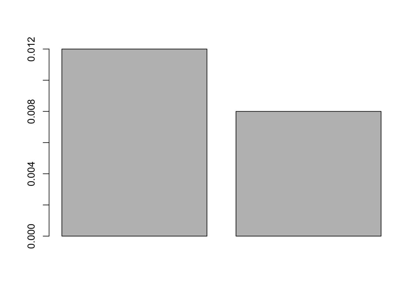
# and we can add extra parameters for nice looking plots
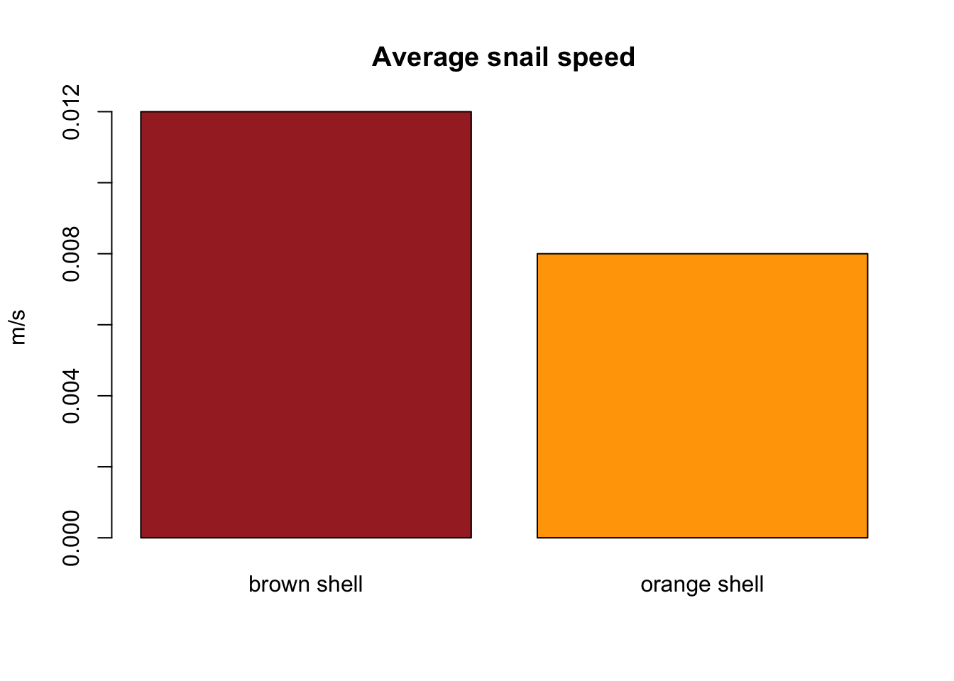
barplot(group_averages$speed, col = levels(group_averages$shell_colour),
main = "Average snail speed", ylab = "m/s", names.arg = c("brown shell", "orange shell"))
if (! require(ggplot2, quietly = TRUE)) {
install.packages("ggplot2")
library(ggplot2)
}
g <- ggplot(data = group_averages)
print(g)
# g with scatter plot (point geometry). Note: no assignment to g object
g + geom_point(mapping = aes(x = shell_colour, y = speed, colour = shell_colour))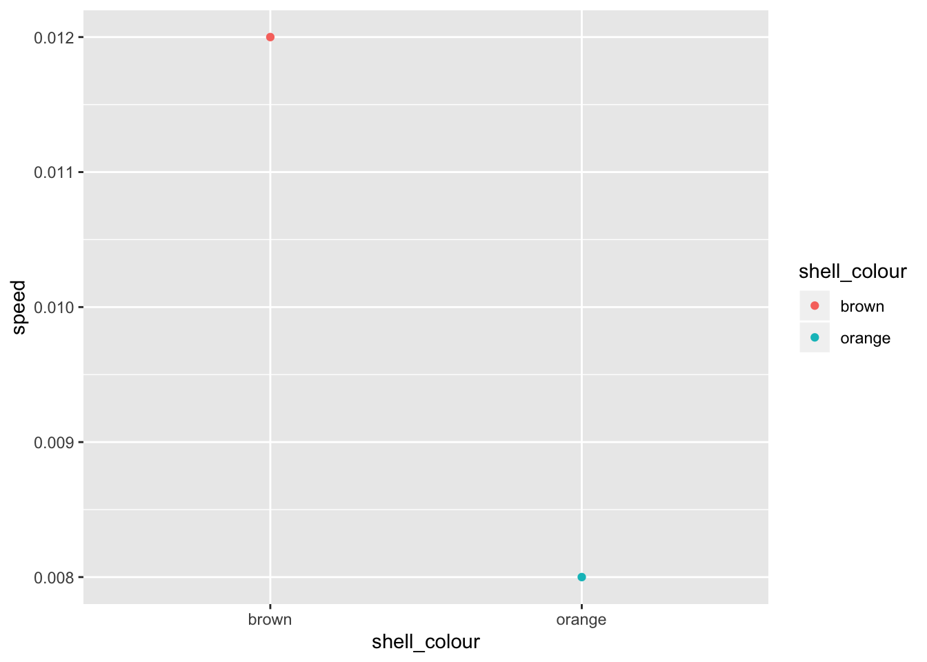
# ggplot objects have additive elements. Note: assignment to g object
g <- g + geom_bar(mapping = aes(x = shell_colour, y = speed, fill = shell_colour),
             stat = "identity")
print(g)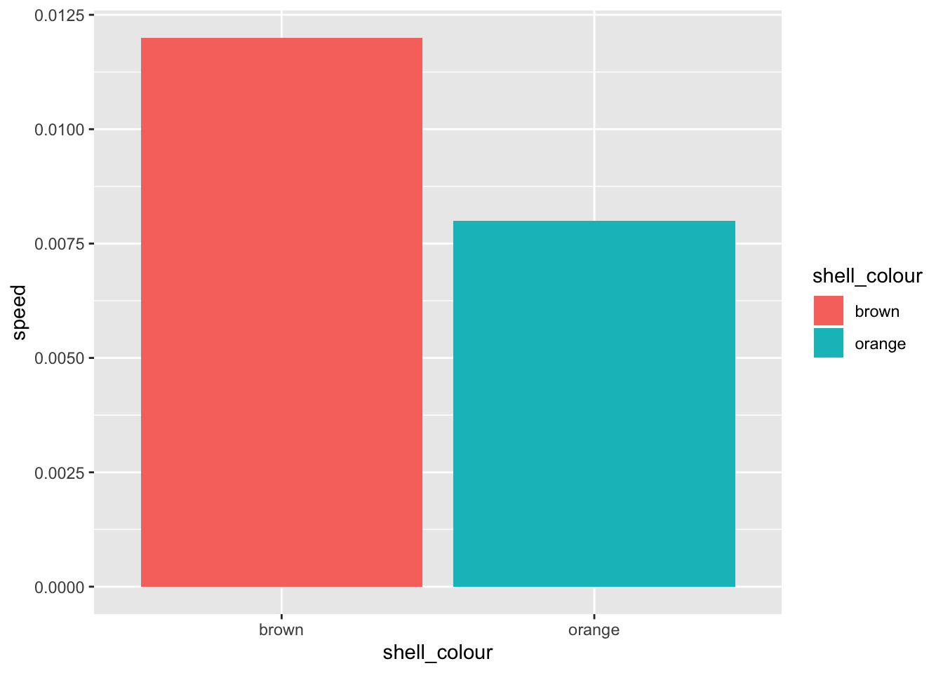
# there are lots of themes and colour pallets to play with. ggplot is very flexible.
g <- g + scale_fill_brewer(palette = "Set1")
print(g)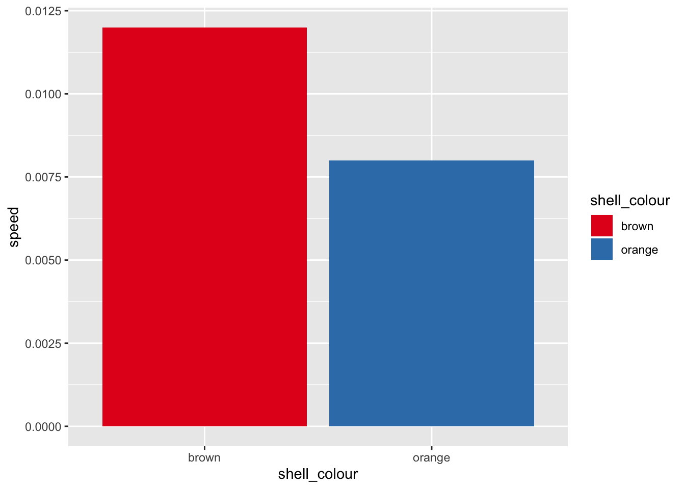
# Adding an element that is already present will override previous settings.

g <- g + scale_fill_manual(values = c("#C4961A", "#D16309"))
## Scale for 'fill' is already present. Adding another scale for 'fill',
## which will replace the existing scale.print(g)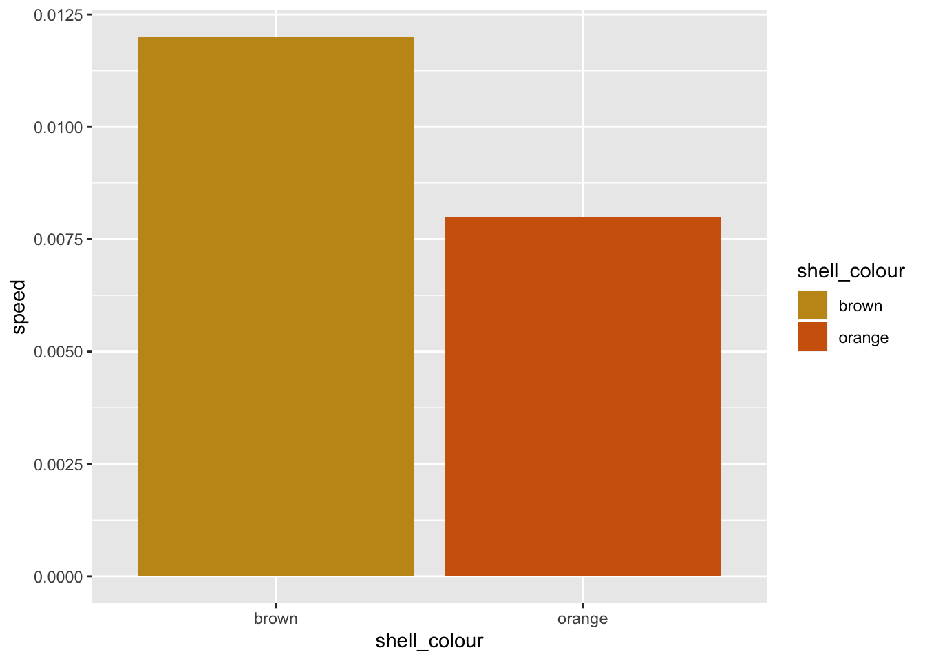
1.8 Scripts
An .R file with no saved output is not generally a useful script. You can press “run”, but you won’t see anything happen. This isn’t because nothing’s happening, but rather the results are not being output to somewhere you can see. We can save plots, or data by writing to files…
# the next few lines save a plot to an image file
png()
barplot(group_averages$speed, col = levels(group_averages$shell_colour),
        main = "Average snail speed", ylab = "m/s", names.arg = c("brown shell", "orange shell"))
dev.off()

# similarly, with ggplot...
g <- g + ggtitle("Avgerage snail speed by shell colour")
ggsave(plot = g, filename = "~/Downloads/ggImage.png")
1.9 More functionality
There are two resources to know for getting the most out of R - CRAN and Bioconductor. Both of these have lots of different packages available, which give you access to functionality that other people have developed. To name a few… - ggplot2 - dplyr - BSgenome - biomaRt
2. Databases
2.1 Getting data
2.1.1 Example: STRING database
2.2 Data manipulation
2.2.1 Subsetting
2.2.2 Data exploration
3. Data-driven conclusions
3.1 Visualization
3.1.1 Set Up
With the STRING data that we downloaded and previewed previously, we will create a network (aka. graph) representing protein interactions, and observe how certain proteins group together in “communities” with shared similarities.
# load an R package that will be useful for our task
if (!require(igraph)) {
  install.packages("igraph")
  library(igraph)
}
## Loading required package: igraph##
## Attaching package: 'igraph'## The following objects are masked from 'package:dplyr':
##
## as_data_frame, groups, union## The following objects are masked from 'package:stats':
##
## decompose, spectrum## The following object is masked from 'package:base':
##
## union# load data from STRING database, prepared in getData.R
load("./data/preparedData.RData")3.1.2 Define functions
We will define a few functions that let us do certain operations on the data.
getGraphSize <- function(G){
  # Find the difference in sizes between the largest
  # and second largest communities in graph G
  # Parameters:
  #   G: an igraph
  #
  # Value: an integer

  # get cluster sizes
  sizes <- sizes(cluster_infomap(G))

  # order sizes as a vector
  sizesOrdered <- as.vector(sizes)

  # in some cases there is only one community
  if (length(sizesOrdered) == 1){
    # in this case, only return this community
    return(sizesOrdered[1])
  }

  # find difference between first and second largest community
  return(sizesOrdered[1] - sizesOrdered[2])
}

randGraph <- function(G){
  # Make a random graph of same degree as an input igraph G
  # Parameters:
  #   G: an igraph
  #
  # Value: an undirected igraph with same degree as G

  d <- degree(G)
  return(sample_degseq(d, method = "vl"))
}
3.1.3 Plot network
This sections is modified from Boris Steipe’s FND-MAT-Graphs_and_networks.R Version 1.0
Create an igraph object from our STRING network, by plotting the network according to community membership of each protein (represented as nodes)
An edge in our network is defined between a pair of proteins. For all the pairs in our dataset, we want to create an edge. We select these as columns 1 and 2 of our prepared dataset.
stringNetwork <- graph_from_edgelist(as.matrix(preparedData[c(1,2)]), directed = F)

# With functions from iGraph package, prepare network for plotting
communities <- cluster_infomap(stringNetwork)
networkLayout <- layout_with_graphopt(stringNetwork, charge = 0.002, mass=100, spring.constant = 0.5)

# Plot!
plot( stringNetwork,
      layout = networkLayout,
      rescale = F,
      xlim = c(min(networkLayout[,1]) * 0.99, max(networkLayout[,1]) * 1.01),
      ylim = c(min(networkLayout[,2]) * 0.99, max(networkLayout[,2]) * 1.01),
      vertex.color=rainbow(max(membership(communities)+1))[membership(communities)+1],
      vertex.size = 700 + (90 * degree(stringNetwork)),
      vertex.label = NA,
      main = "Network from STRING data"
    )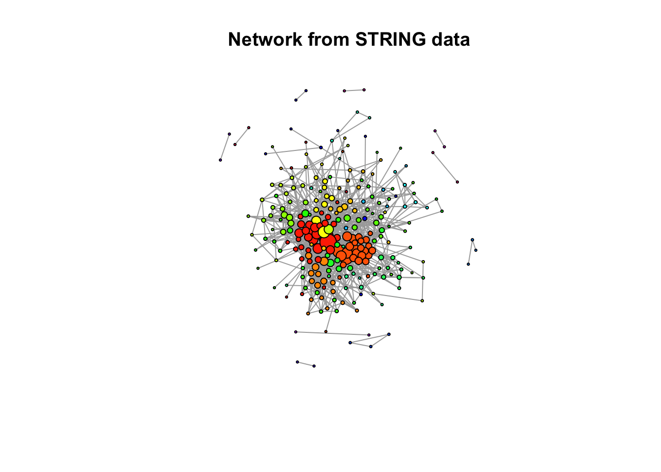
With these settings, size of a node increases with degree, colour is dictated by community membership. We can see that there are several fairly well connected nodes with high degree of connectivity to other nodes. These nodes tend to be members of larger communities - this makes sense biologically, we could expect a protein in a large group of interacting proteins has many interactions. There are two distinctly large and well connected communities.